Control Notes

Background

A few weeks ago, a refinery got me out to tune the control loops on their thermal oxidizer. A thermal oxidizer (TOX) is a specialized combustion system that uses heat to destroy volatile organic compounds (VOCs) and hazardous air pollutants so that they aren’t released into the atmosphere.

This particular TOX had two distinct control modes, hot-standby and in-service. Its heat source was natural gas and it had one gas-flow control valve that was used in hot-standby mode and another, larger control valve for when the TOX was in service. The TOX had an outlet temperature control loop that was particularly problematic.

The refinery’s issue with the outlet temperature control was that its response was extremely sluggish in hot-standby mode, struggling to maintain TOX temperature and frequently causing trips on high temperature, especially when transitioning from in-service to hot-standby mode.

The TOX had an outlet temperature controller that manipulated the setpoint of a cascaded gas-flow controller to control temperature. In turn, the gas-flow controller manipulated the two gas-flow control valves to control the gas flowrate using split-range control.

Spit-Range Control

Split-range control is a common advanced regulatory control (ARC) design used when a single controller must manipulate two (or more) control valves. Typically, the valves have different trim sizes with one valve being smaller and used for low-flow conditions such as process startup, and the other valve being larger and used for controlling higher flowrates.

Figure 1 shows an example of a split-range control design that uses two function generators, also known as f(x) function blocks, to split the controller’s output between the two valves.

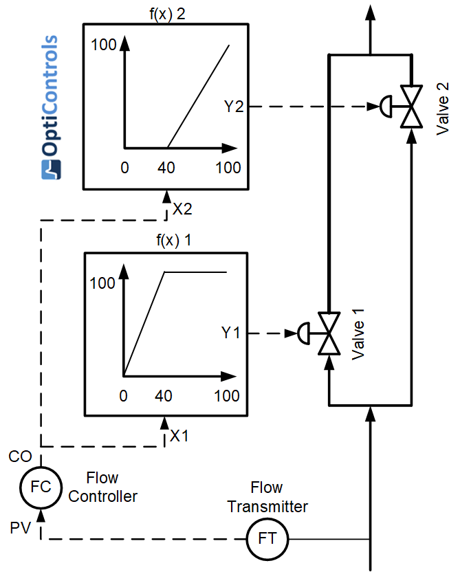
The Split Point

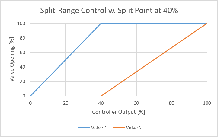
The split point defines the percentage controller output where the first valve is fully open and the second valve is still closed but ready to open if the controller output increases. Figure 2 illustrates the operation of a split-range design with a split point of 40%. Valve 1 opens from 0% to 40% controller output and Valve 2 opens from 40% to 100% output.

Although rarely correct, most split-range control designs have their split points configured to be at 50%. This is wrong because the split point should be used to compensate for the difference in valve sizes to balance or equalize the process gain across both valves. Smaller control valves have less effect on the process (lower process gain) and should be opened faster to compensate, while larger control valves have more effect on the process (higher process gains) and should be opened slower to compensate.

The correct split point can be calculated using Equation 1 below.

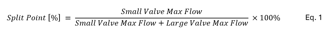
Max Flow in Equation 1 means the respective flowrates of the valves at 100% open. One could also use the flowrates at other large valve openings, such as 75% or 50%, as long as both valves are at the same percentage open when the flowrate is measured. Alternatively, the two valves’ flow coefficients (Cv) at 100% open can be used instead of the maximum flowrates in Equation 1. The max Cv can be obtained from the manufacturer, from the valves’ data sheets, or by using valve sizing software.

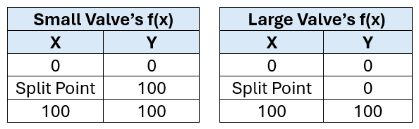
Once the split point has been determined, the X-Y pairs in the two function generators or f(x) blocks can be configured as shown in Table 1 below.

Table 1. Function generator configuration.

Back to the TOX

As stated above, the two gas valves on the TOX had different sizes. However, the split point was at 50%, i.e. 0% to 50% controller output opened the small control valve and 50% to 100% opened the large control valve. By doing a few well-orchestrated flowrate tests and subsequent calculations, the flow curves of the two valves were determined. These are shown below in Figure 3.

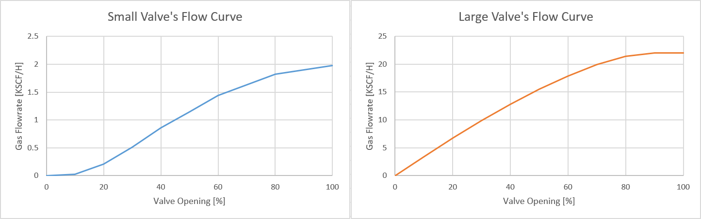
The two flow curves look reasonably similar in Figure 3 (except for the flat region at the low end of the small valve) but their Y-axis (flowrate) scales are different by almost an order of magnitude. If the combined, total flowrate is charted, a different picture emerges, as shown in Figure 4. Now it becomes clear that the small valve has a very flat flow curve (low process gain) compared to the large valve that has a steep flow curve (high process gain).

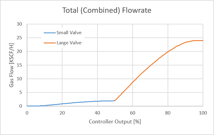
A PID controller cannot produce acceptable performance when the process gain varies this much over the operating range. The TOX’s outlet temperature controller was tuned with the large valve in control, hence the poor performance when the small valve came into play.

Using Equation 1 and the two control valves’ respective flow rates at 70% open (to disregard the flatness of the flow curves at the high end), the ideal split point was calculated to be 7.5%. If the flowrates at 100% were used, the split point amounted to 8.2%, which is in the same ballpark (about 10% more). The new combined, total flowrate of the two valves, using the correct split point is shown in Figure 5.

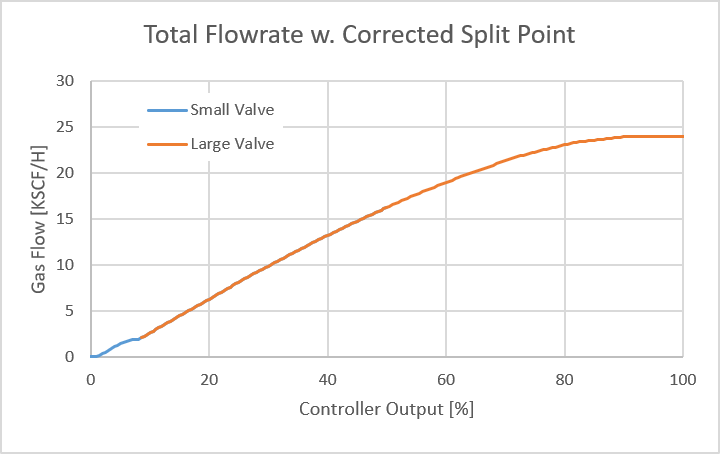
When using the correct split point of 7.5%, the flow gradients of the two valves are very similar and vastly improved over using a split point of 50% as shown in Figure 4.

Implementation

The two function generators, that were already present in the control design, were reconfigured to correct the split-point to 7.5%. The operator graphic was updated to indicate that the small valve now opens between 0% and 7.5% controller output and the large valve opens between 7.5% and 100%. After the new split point was implemented, the flow control loop’s PID controller was retuned and control response was tested in hot-standby and in-service modes.

Future Improvement

If needed, valve characterization could have been used to deal with the nonlinear valve curves shown in Figure 3, but the small valve rarely operated below 30% open and the large valve never opened more than 60% under normal operating conditions, so it was decided to keep the design simple and forego the additional linearization.

Results

Overall, after correcting the split point, the performance of the temperature control loop was very good throughout the entire operating range and the TOX did not trip on high outlet temperature anymore.

Stay Tuned!
Jacques – Author of Process Control for Practitioners.