Super-High Controller Gains
Controller gains of properly tuned loops are typically within the range of 0.1 to 10. During my process control training workshops, I advise participants to be careful when applying controller gains greater than 10 – even when a tuning rule recommends it. The reason why I recommend this is that changes in the error signal (difference between the Process Variable and the Setpoint) are multiplied by the controller gain and sent to the controller output.
For example, if the process variable signal contains 1% of noise and the controller gain is set to 10, the controller output signal will contain 10% noise. This means that the control valve will receive these large changes in position demand at a very high rate – leading to excessive control valve wear and possibly to large process disturbances too. (Note that this can be alleviated by using a process variable filter if the frequency of the noise is high, with the downside of slowing down the loop’s response).
Also, if an operator makes a 5% setpoint change on a controller with a gain of 10, the controller output will attempt to jump 50%, often fully opening or closing the control valve. (Note that this can be prevented by configuring the controller to let proportional and derivative modes act only on changes in process variable; not on setpoint changes).
However, some control loops require controller gains much larger than 10 for good control. Two examples follow.
Highly Lag-Dominant Processes
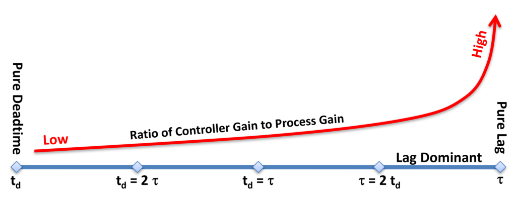
I explained in a previous post on deadtime versus lag that there is a continuum from processes with pure deadtime to processes with pure lag. The closer a process comes to being a pure lag, the higher the recommended controller gain will be. A good starting point for controller gain to use on a lag-dominant process is:
Controller Gain = (Time Constant) / (2.5 x Process Gain x Deadtime)
You can see from this equation above and the figure below that the more lag-dominant a process is (i.e. the larger the ratio of time constant to deadtime), the higher the controller gain should be.

Note: Processes that are highly lag-dominant are often better modeled and tuned as integrating processes. Still, the modeled integration rate of the process will be very low, again requiring the use of a high controller gain for good control.
One type of process that is highly lag-dominant and calls for super-high controller gains is large-volume, gas-pressure systems. These processes typically have relatively short deadtimes and very long lags (time constants). If such a process also has minimal noise on the process variable signal, the use of a super high controller gain is justified, and often required for good control. The highest controller gain I have personally used on such a system was 45. It was for a pressure control loop on an H2S stripper in a sour water plant.
Very Low Process Gains
Another type of process that typically requires using super-high controller gains is those with a very low process gain. From the equation for controller gain given above, you can see that controller gain is proportional to the reciprocal of process gain. This means that the lower the process gain is, the higher the controller gain should be. While process gains of self-regulating processes typically fall within the range of 0.5 to 5, some processes can have extremely low gains. This may be due to the design of the process, but it is more likely to result from the process variable’s signal span (calibrated range of the transmitter) being much wider than the normal operating range of the process.
One of the most extreme cases I have experienced in this regard was a pressure control loop on a vacuum tower in which the pressure (vacuum) transmitter was calibrated to the full range of 0 to 760 mmHg, while the process normally operated in the range of 0 to 15 mmHg. The process gain calculated from step-test data was 0.0087, which required using a super-high controller gain. The process was also lag dominant, further increasing the required controller gain. The controller gain was calculated to be 228. This gain may appear to be extremely high and therefore incorrect, but it worked just fine in the control loop. Since there was a small amount of noise on the measurement signal, I also used a 10-second process variable filter to smooth down controller output movements.

To put things in perspective, the normal operating range (0 – 15 mmHg) was only a small fraction of the transmitter’s calibration range (0 – 760 mmHg); 0.0197 to be exact.
Had the transmitter been calibrated for the operating range, the process gain would have been 0.0087 / 0.0197 or 0.44, which is close to the typical process gain range stated before. Also, the controller gain would have been 228 x 0.0197 or 4.5, which falls within the typical range for controller gains given at the beginning of this article.
Conclusion
The controller gain should be set according to the reciprocal of process gain and the ratio of lag to deadtime. All three of these parameters can be determined easily through step tests. Trial-and-error tuners will very unlikely ever use gains as high as I described in this article.
Also, if you use high controller gains in controllers that are subject to operator-induced setpoint changes, be sure to configure the controller to let proportional and derivative modes act only on changes in process variable; not on setpoint changes.
Stay Tuned!
Jacques – author of Process Control for Practitioners