Overview

Gain-Anchored Tuning (GAT) is a PID tuning method for integrating processes, developed by Jacques Smuts of OptiControls. It is particularly suited for level control in large tanks, vessels, and reservoirs with slow process dynamics.

Traditional tuning methods calculate controller gain based on process dynamics and often produce excessively high gain values for slow-responding processes, especially levels. In these cases, GAT allows the user to select a practical and reasonable controller gain, after which the required integral time is calculated to achieve stable, well-damped control.

The Problem with Conventional Tuning

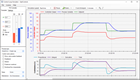
Integrating processes with very long residence times (i.e., very low integration rates) present a challenge in PID controller tuning. Conventional tuning methods (e.g., Lambda or Ziegler–Nichols) often produce excessively high controller gains, resulting in increased sensitivity to measurement noise which causes excessive valve movement (Figure 1).

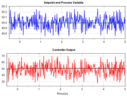
For example, consider a level loop on a large vessel with a residence time of 90 minutes, corresponding to an integration rate of 0.011 min⁻¹. Assuming a dead time of 1 minute, the unmodified Ziegler–Nichols tuning rules yield a controller gain (K_C) of 82 and an integral time (T_I) of 3.3 minutes. (Abbreviations with descriptions are listed at the end of this post).

While mathematically valid, such high controller gains are impractical in real plant operation and typically result in overly aggressive control and increased valve wear.

Changing only K_C

An experienced control engineer would recognize that a controller gain of 82 (from the previous example) is impractical and may reduce it to a more reasonable value, such as 5. However, changing only K_C introduces a new problem: the control loop may exhibit slow, sustained oscillations following a disturbance.

This occurs because reducing the controller gain without adjusting the integral time results in excessive integral action relative to the proportional action. The imbalance causes the controller to overcorrect over time, leading to oscillatory behavior (Figure 2).

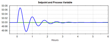
This highlights the need to adjust the integral time in proportion to the selected controller gain.

The Gain-Anchored Tuning Approach

The Gain-Anchored Tuning method alters the traditional tuning workflow for integrating processes. Instead of calculating the controller gain, the user specifies it, and the method determines the appropriate integral time.

This approach allows the control engineer to:

• Select a moderate, robust controller gain (e.g., K_C = 5–10)
• Avoid excessive controller aggressiveness and noise sensitivity
• Maintain intuitive control over the loop response

The Gain-Anchored Tuning Method

The Gain-Anchored Tuning method applies to integrating processes with dominant integrating behavior, typically characterized by a residence time that is at least 10 times greater than the process dead time (i.e., t_res ≥ 10 θ).

For integrating processes, the controller gain (K_C) or proportional gain (K_P) is specified by the user and then the integral time (T_I) or integral gain (K_I) is calculated as:

For Standard Controller Form	For Parallel Controller Form
TI = M tres / KC or equivalently: TI = M / (ri KC)	KI = KP2 / (M tres) or equivantly: KI = KP2 ri / M

where:

• K_C = controller gain (user-specified)
• K_P = proportional gain (user-specified)
• T_I = integral time
• K_I = integral gain
• t_res = process residence time
• r_i = process integration rate
• M = tuning factor, or moderation factor, (typically between 2 and 4)

The tuning factor M adjusts the closed-loop response:

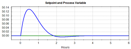
• M = 2: moderately fast response with some overshoot following a disturbance (Figure 3)
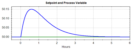
• M = 4: well-damped response with no overshoot (Figure 4)

Determining r_i and t_res

The integration rate (r_i) of an integrating process can be determined by putting the controller in manual and making a step change in the controller output. For best accuracy, the output step should be large enough to produce a clear change in process variable (PV) slope, but small enough to avoid operating constraints.

Measure the slope of the PV before and after the step (in %/minute), subtract the initial slope from the final slope, and divide the result by the magnitude of the output step change.

A more detailed description is available here: https://blog.opticontrols.com/level-control-loop-tuning/

The residence time of a vessel (t_res) can be estimated by dividing the working volume of the vessel (corresponding to 0–100% level) by the maximum flow rate through the final control element (e.g., control valve or variable-speed pump).

Note that integration rate and residence time are reciprocals, meaning that residence time can be calculated from integration rate (and vice versa):

t_res = 1/r_i.

Typical Application: Level Control

Gain-Anchored Tuning is particularly well suited for:

• Tank level control
• Surge vessels
• Liquid (e.g., water) reservoirs
• Any process with dominant integrating behavior (t_res ≥ 10 θ)

In these applications:

• Stability and smooth operation are more important than speed
• Excessive gain leads to unnecessary valve movement and wear
• Operators prefer predictable, smooth, and non-oscillatory behavior

Example

Consider the vessel with a long residence time used previously:

• t_res = 90 minutes, deadtime (θ) = 1 minute
• Ziegler-Nichols tuning produced K_C = 82, T_I = 3.33

The K_C of 82 is impractical. If it is reduced to 5, the T_I of 3.33 is much too fast and causes oscillations.

Using Gain-Anchored Tuning:

• Still choosing K_C = 5 (practical, robust)
• Then using M = 4, GAT renders T_I = 72 minutes

This results in:

• Stable, well-damped control
• Reasonable controller output movement
• Improved robustness to disturbances and noise

Key Advantages of Gain-Anchored Tuning

• Prevents unrealistically high controller gains
• Improves robustness and operability
• Gives the user intuitive control over loop behavior
• Well suited for slow integrating processes
• Simple and transparent tuning relationship

Summary

Gain-Anchored Tuning provides a practical and effective alternative to conventional tuning methods for integrating processes. By basing the design on a user-selected controller gain, Gain-Anchored Tuning avoids the excessive aggressiveness often produced by traditional methods, and delivers stable, well-damped control performance in real-world applications.

Acronyms and Abbreviations

GAT	Gain-Anchored Tuning
KC	Controller Gain
KI	Integral gain
KP	Proportional Gain
M	Gain-Anchored Tuning Factor (Moderation Factor)
PID	Proportional + Integral + Derivative (Control)
Pk-Pk	Peak-to-Peak
ri	Integration Rate
θ	Deadtime
PV	Process Variable
TI	Integral Time
tres	Residence Time

Credit
The author acknowledges that the Gain-Anchored Tuning method was derived from Greg McMillan’s recommendations for stability of integrating control loops.

Stay tuned!
Jacques – Author of Process Control for Practitioners.