Control Notes

When you push down on your car’s accelerator, you expect the car to speed up, right? What if it slows down? Or even worse: You lift your foot off the accelerator and your car speeds up. And the more you lift your foot, the more the car speeds up. These are almost unthinkable and certainly scary situations, yet they occur every day in thousands of boilers and some other processes around the world. The phenomenon is called an inverse response. One of the most common occurrences of inverse response is found in the control of boiler drum level.

Boiler Drum Level Control

In a boiler, water is converted to steam. Steam and water separates in the boiler drum, with the steam then leaving through a pipe at the top of the drum. It is important to keep the level of water in the drum away from this pipe or water will exit with the steam and damage downstream equipment. Even more important is to always have some water in the drum – when the boiler runs dry there is no water to cool it, and this will result in severe damage to the boiler. So the water level in the drum is normally maintained close to its centerline.

The drum level is controlled by adding water to the boiler, called feedwater. A closed-loop controller looks at the drum level and if it is lower than the setpoint it opens the feedwater control valve to increase the feedwater flow rate and vice versa (Figure 1). This brings us to inverse response…

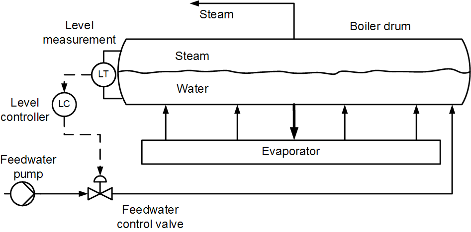
Figure 1. Boiler drum level control diagram.

Inverse Response

The temperature of the feedwater flowing into the drum is normally below boiling point. When we add more of this colder water to the boiler, some of the steam bubbles in the boiler condense. This causes the drum level to decrease and the effect is called inverse response. However, the effect is only temporary. After a while, the higher rate of feedwater flow overcomes the lost volume and the drum level rises (Figure 2). The opposite is also true: when we decrease the flow rate of the colder feedwater, steam production increases, and the additional steam bubbles cause the drum level to rise. But after a while, the drum level begins to fall, as expected.

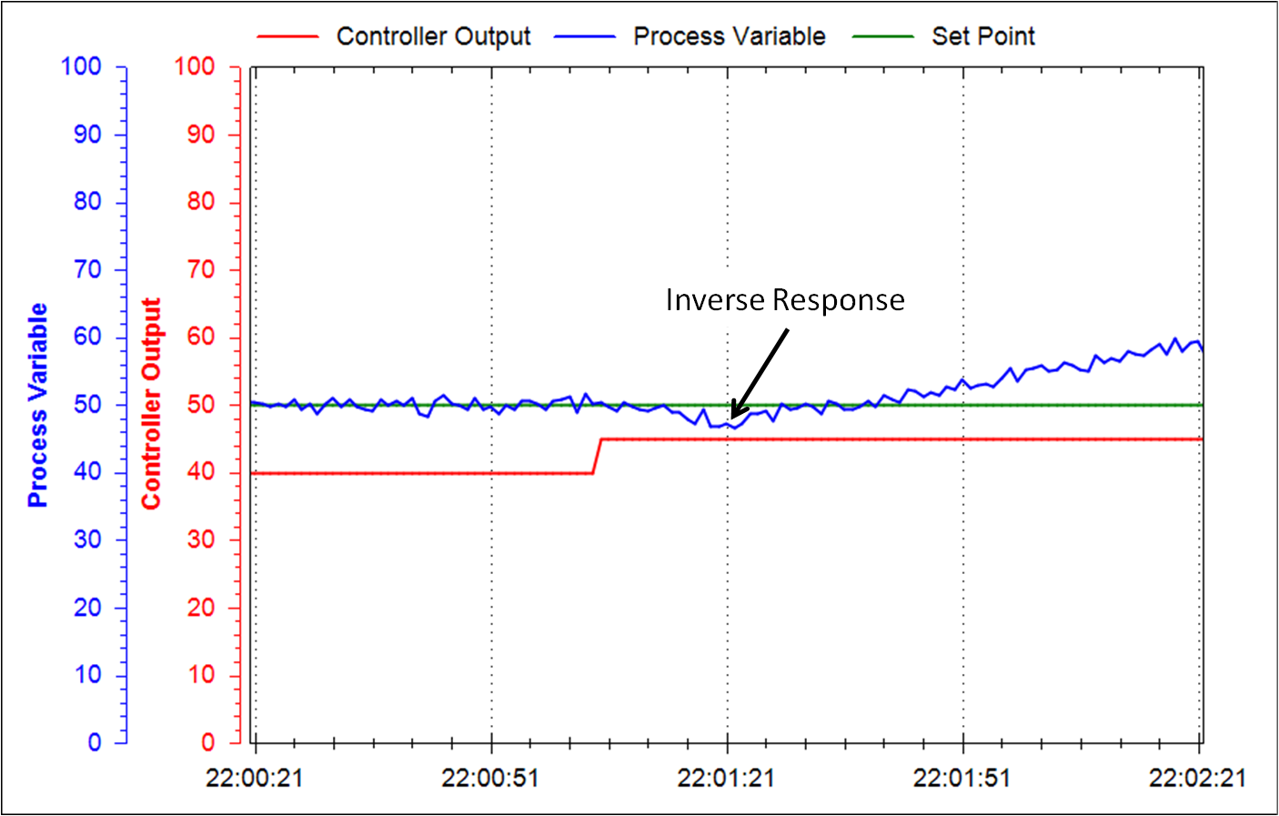
Figure 2. With inverse response, the process first responds in the wrong (inverse) direction, and then in the expected direction.

I have not seen many other processes exhibiting inverse response. Two that come to mind are distillation column bottom level control (very similar to drum level control) and crystal size control in certain crystallizers (see case study below).

Tuning Implications

Processes exhibiting inverse response can easily cause control loop stability problems. Using derivative control is questionable from a stability perspective, and certainly not useful. Using a high controller gain is not possible since it will “chase” the inversely responding process and create a snowball (runaway) effect. But when you use a low controller gain on an integrating process, you also have to use a long integral time (low integral gain). So you end up with a very slow-responding control loop, and any attempt to speed it up significantly lowers its stability. This is why three-element control is the strategy of choice for drum level control.

When you do step-testing on a process with an inverse response and determine the process characteristics to tune the controller, you should treat the entire duration of the inverse response as dead time (Figure 3). Then you can apply your usual level controller tuning rules using this pseudo dead time.

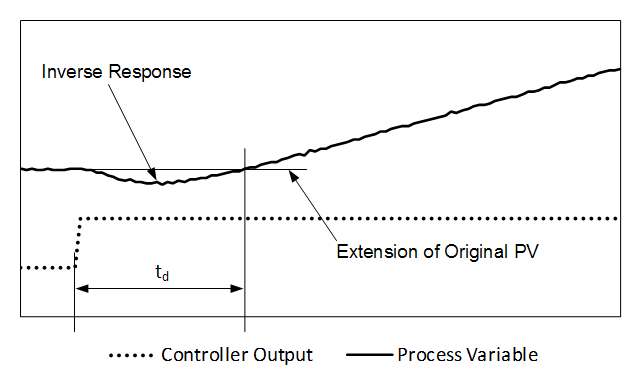
Figure 3. Dead-time (td) measurement on an inversely responding process.

Case Study

Below is an example of dealing with inverse response in a different process.

A few weeks ago I was optimizing control loops on an ammonium sulfate crystallizer. The crystal size was very important, but it could not be measured directly. Instead the agitator motor amps were used as an indication of crystal size. Control was done by changing the feed rate of saturated liquid to the crystallizer, thereby changing the residence time of slurry in the crystallizer, and subsequently changing the crystal size. However, changes in feed rate also changed the crystallizer level, which turned out to cause a profound inverse response on the agitator amps because of the mechanical design of this particular crystallizer. The plant personnel was unaware of this, but the inverse response was revealed when we did step-testing.

The control was rather poor before we got started. There were large oscillations in motor amps, caused by large variations in crystal size. After step-testing, we calculated the new controller settings, recorded a week of data as a baseline (because we increased the process historian’s sampling resolution), and then entered the new settings. A time-trend of the control performance before and after tuning is shown in Figure 4.

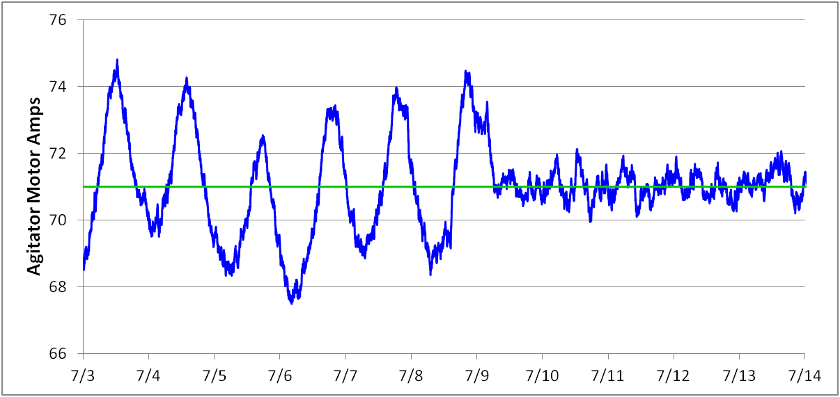
Figure 4. Improvement in control of an inversely-responding process through proper tuning. New tuning settings were entered during the morning of 7/9. Blue = motor amps; Green = setpoint.

Needless to say, the production manager was very happy with the control improvement and the plant is now selling the ammonium sulfate crystals at a higher price because of the improvement in quality.

Stay tuned!

Jacques Smuts
Principal Consultant at OptiControls, and author of Process Control for Practitioners.