5. Control Valves
Control Valve Response Time
For a long time I suspected that control valves take longer to respond to small changes in controller output than to large ones. I have now confirmed this by doing tests on several control valves and analyzing the results.
Most of my control loop optimization work has been on live running processes, so I never had the chance to really confirm or disprove my suspicion. I can rarely make 10% or larger step changes in controller output because that will upset the processes far too much. Also, most of the plants I have been working at do not have valve-position feedback readily available for recording/analysis, and many processes respond so slowly relative to a valve’s response time that the latter is immeasurable from the process response.
This all changed a while ago when I became involved with the startup of a large new chemical plant. As we commissioned individual pieces of equipment and subsystems, I had opportunities to do tests I will never get to do on a live running process. The control valves I included in this analysis were all gas-flow control valves that had high pressure differentials (DP) across them, so valve movement had a direct and almost instantaneous effect on the measured gas flow rate. Also, all the valves had position feedback to the DCS via HART communications, making this data readily available through OPC for recording and analysis.
Most of the control valves were globe valves, but a few of them were butterfly valves. The valves ranged between 2” and 24” in size. Most of them had diaphragm actuators, but some had piston actuators. The valves all had smart positioners (digital valve controllers) that were tuned by OEM technicians using valve calibration software. The larger control valves were fitted with volume boosters to increase the air flow rate to their actuators, allowing them to travel full stroke within a few seconds.
As part of my normal control loop diagnostic and tuning activities, I always test the performance of the final control element (control valve, damper etc.), if possible. During this startup project, I did a few additional step changes to determine the dynamic response of the target group of control valves over a range of step-change sizes, typically 0.5%, 1%, 2%, 5%, 10% and 25% (Figure 1).
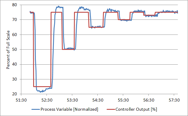
Figure 1. A typical sequence of steps to analyze control valve response time. (Click to enlarge.)
Although the plant had position feedback signals from all its valves, I did not want to rely on the non-deterministic speed of HART communications. Since the gas flow rate changed virtually instantaneously with valve position, I used this as my primary indication of when the valve actually responded and used the valve position feedback solely for validation. I used control loop tuning software to determine the actual dead time from the process response curve – this gave me higher resolution than the scan time of the DCS.
The test results showed that the time delay (dead time) between the controller output signal changing and the control valve responding, increased inversely with step-change size. In other words, most control valves took remarkably longer to respond to small changes in controller output than to large changes. For step sizes of 10% or greater, the dead time remained virtually unchanged. But for step sizes less than 10% in size, the dead time increased significantly as the step changes became smaller (Figure 2). The same was not true for the control valves’ average time constant, which remained relatively unchanged at smaller step sizes.
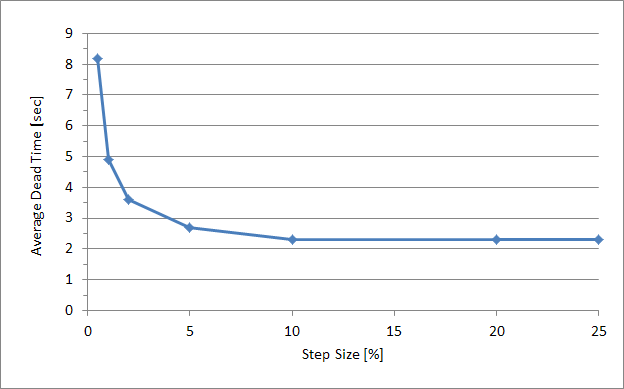
Figure 2. Dead time increasing at small step sizes.
Impact on Tuning
Since controller tuning settings are based on the dead time in the process (among other things), increases in dead time can have serious effects on control loop stability.
Fortunately most control loops should not be affected by this increase in dead time. This is because the dynamic response of most processes is much slower than the dynamics of the control valves, and an increase in dead time will go virtually unnoticed. However, for processes with a super-fast response, such as liquid pressure and gas flow, one should take this creep in dead time into account when tuning control loops. Fast-responding liquid flow control loops could also be subject to this problem.
Let’s consider tuning one of these fast-responding processes. You do step tests of 5% in size and calculate the dead time, time constant, and process gain. Then you use a suitable tuning rule (such as the modified Cohen-Coon tuning rules) to calculate tuning parameters for the controller. After you implement the new settings, you test the control response by making a 5% change in setpoint. And all seems well. However, once the process settles back into normal operation, the controller output changes only a fraction of a percent at a time and the increased dead time results in a small, persistent limit cycle (oscillation). The control loop is simply not tuned to handle the now longer dead time.
You could recalculate your tuning settings based on a longer dead time. This will result in a lower controller gain and a longer integral time. The new tuning settings may settle down the control loop, but at the price of sacrificing loop performance. As the controls practitioner, you will have to make the call what the optimum tuning settings are, based on the process’ sensitivity to oscillations versus the impact of slower response to setpoint changes or disturbances.
Stay Tuned!
Jacques Smuts
Author of Process Control for Practitioners