1. General
Controller Tuning Objectives
Controller tuning is a mystery to most people who do not have firsthand experience with it. A process engineer recently asked me how I would know what speed of response his control loops should be tuned for. Using the analogy of guitar tuning, he asserted that if a control loop is not tuned for the perfect speed of response, it will be out of harmony with the rest of process, just as a guitar will be out of tune if its strings are not all tuned to their own perfect pitch. This is not how it works in practice.
There is no need to know upfront the exact speed every control loop should be tuned for. The purpose of an automatic controller is to keep the process close to its given setpoint. It is therefore reasonable to expect that most control loops should, after setpoint changes and disturbances, respond quickly to bring the process back to setpoint in a fast manner.
Let’s briefly explore the concept of “fast” response. I am a marathon runner (Figure 1) and my average finishing time is around 4 hours. For me, a fast marathon would have a personal finish time of 3:50. For an Olympic marathon runner, a fast finish time would be 2:10. Every runner’s personal concept of running fast depends on his/her own capabilities. Similarly, every control loop’s concept of responding fast depends on the dynamics of the process it is controlling. For example: a “fast” kiln temperature control loop could respond orders of magnitude slower than a fast flow control loop. A fast loop response is relative to the dynamics (dead time and lag) of its process.

Figure 1. The author running a marathon.
However, simply tuning control loops for their fastest possible speed of response (e.g. using quarter-amplitude damping tuning methods) renders control loops oscillatory and very sensitive to changes in process dynamics. Hence, control loops should be tuned for a slightly slower response than maximum speed to obtain a balance between speed of response and robustness/stability. Using the modified Cohen-Coon tuning rules with a stability margin of 2.5 or 3 is an appropriate tuning method for most control loops. So, for the majority of control loops you don’t need to know the target speed of response up front. You simply have to use the right tuning method.
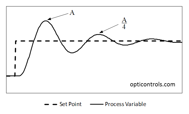
Figure 2. Tuning for quarter-amplitude damping leaves a loop oscillatory and very vulnerable to changes in process conditions.
There are cases in which control loops have to be tuned for a slower and/or more stable response. These include control loops on highly interactive processes (e.g. pressure-reducing and flow-control valves in series) and loops that can disturb sensitive processes if their outputs change too fast (e.g. surge tank level control). These cases can be identified by studying the process design, asking process engineers, or talking to operators. Find out what gets disturbed if the controller output changes too rapidly, and then determine an appropriately slow response for the control loop based on the speed of recovery of the process/control loop it is disturbing. The Lambda and Level-Averaging tuning rules are normally appropriate tuning rules for these loops.
Some processes cannot tolerate any overshoot after setpoint changes. Overshoot after a setpoint change is more prevalent on lag-dominant loops such as temperature and gas-pressure control. These loops should still be tuned for a balanced (i.e. fast) response to handle process disturbances. The no-overshoot requirement should then be addressed with setpoint filtering (i.e. passing the setpoint through a first-order lag, as shown in Figure 3). Note that a level control loop will always overshoot after a setpoint change, unless the controller’s integral term is disabled until the new setpoint is reached.
If the process needs to slowly and gradually move from one operating point to the next, the previous paragraph still applies, but instead of a setpoint filter, the setpoint needs to be ramped to its new value at the rate specified by the process design, as shown in Figure 3.
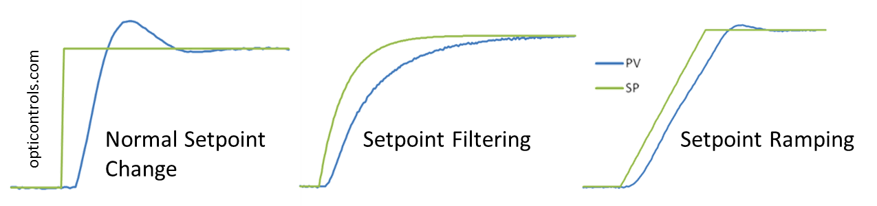
Figure 3. Setpoint filtering to prevent overshoot after a setpoint change, and setpoint ramping to obtain a specific rate of change. (Click to enlarge)
You can use the OptiControls Loop Simulator software to demonstrate most of the process control fundamentals discussed in this article, and read more about them in the book Process Control for Practitioners.
Stay tuned,
Jacques Smuts, Ph.D., P.E.
Founder and Principal Consultant
OptiControls Inc.